An Intuitive Introduction Of Restricted Boltzmann Machine (RBM)

Introduction

RBM is a variant of Boltzmann Machine, RBM was invented by Paul Smolensky in 1986 with name Harmonium. In the mid-2000, Geoffrey Hinton and collaborators invented fast learning algorithms which were commercially successful.

• RBM can be use in many applications like Dimensionality reduction , Collaborative Filtering, Feature Learning, Regression Classification and Topic Modeling.
• It can be trained in either Supervised or Unsupervised ways, depending on the task.

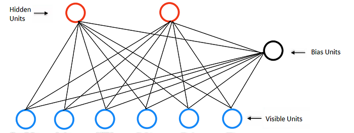
RBM’s Architecture

• This Restricted Boltzmann Machine (RBM) have an input layer (also referred to as the visible layer) and one single hidden layer and the connections among the neurons are restricted.
• Neurons are connected only to the neurons in other layers but not to neurons within the same layer.
• There are no connections among visible neurons to visible neurons.
• There are no connections among hidden neurons to hidden neurons.
• In RBM visible and hidden neurons connections form a bipartite graph.
• An RBM is considered “restricted” because no two nodes in the
  same layer share a connection

Restricted Boltzmann Machine

How does RBM work?

RBM has two phases

• Forward Pass
• Backward Pass or Reconstruction

RBM takes the inputs and translates them to a set of numbers that represents them(forward pass). Then, these numbers can be translated back to reconstruct the inputs(backward pass).

In the forward pass, an RBM takes the inputs and translates them into a set of numbers that encode the inputs.

In the backward pass, it takes this set of numbers and translates them back to form the re-constructed inputs.

Machine Learning in Finance - Data Driven Investor

Through several forward and backward passes, an RBM is trained to reconstruct the input data. Three steps are repeated over and over through the training process.

(a) With a forward pass, every input is combined with an individual weight and one overall bias, and the result is passed to the hidden layer which may or may not activate.

(b) Next, in a backward pass, each activation is combined with an individual weight and an overall bias, and the result is passed to the visible layer for reconstruction.
(c) At the visible layer, the reconstruction is compared against the original input to determine the quality of the result.

A trained RBM can reveal which features are the most important ones when detecting patterns.

A well-trained net will be able to perform the backwards translation with a high degree of accuracy. In both steps, the weights and biases have a very important role. They allow the RBM to decipher the interrelationships among the input features, and they also help the RBM decide which input features are the most important when detecting patterns.

An important note is that an RBM is actually making decisions about which input features are important and how they should be combined to form patterns. In other words, an RBM is part of a family of feature extractor neural nets, which are all designed to recognize inherent patterns in data. These nets are also called autoencoders, because in a way, they have to encode their own structure.

Note : RBMs use a stochastic approach to learning the underlying structure of data, whereas autoencoders, for example, use a deterministic approach.

Understanding RBM with an example

Let’s take an example, Imagine that in our example has only vectors with 7 values, so the visible layer must have j=7 input nodes. The second layer is the hidden layer, which possesses i neurons in our case, we will use 2 nodes in the hidden layer, so i = 2.

Each hidden node can have either 0 or 1 values (i.e. si = 1 or si = 0) with a probability that is a logistic function of the inputs it receives from the other j visible units, are called p(si = 1).

Each node in the visible layer also has a bias. We will denote the bias as “v_b” for the visible units. The v_b is shared among all visible units.

We also define the bias for the hidden layer as well. We will denote this bias by “h_b” . The h_b is shared among all hidden units.

import tensorflow as tf
v_b = tf.placeholder(“float”, [7])
h_b = tf.placeholder(“float”, [2])

We need to define weights among the visible layer and hidden layer nodes. In the weight matrix, the number of rows are equal to the visible nodes, and the number of columns are equal to the hidden nodes.

Let W be the tensor of 7x2, where 7 is the number of neurons in visible layer and 2 is the number of neurons in hidden layer.

W = tf.constant(np.random.normal(loc=0.0, scale=1.0, size=(7, 2)).astype(np.float32))

Forward Pass : One training sample X given as a input to all the visible nodes, and pass it to all hidden nodes. Processing happens at each hidden layer’s node. This computation begins by making stochastic decisions about whether to transmit that input or not (determine the state of each hidden layer). At the hidden layer’s nodes, X is multiplied by a 𝑊𝑖𝑗 and added to h_b. The result of those two operations is fed into the sigmoid function, which produces the node’s output, p(hj), where j is the unit number.

p(hj) is the probabilities of the hidden units. And all values together are called probability distribution. RBM uses inputs X to make predictions about hidden node activation. For example, imagine that the values of ℎp for the first training item is [0.51 0.84]. It tells us what is the conditional probability for each hidden neuron to be at Forward Pass:

• p(ℎ1 = 1|V) = 0.51
• p(ℎ2 = 1|V) = 0.84

As a result, for each row in the training set, a vector/tensor is generated, which in our case it is of size [1x2], and totally n vectors (𝑝(ℎ)=[nx2]).

We then turn unit ℎ𝑗 on with probability 𝑝(ℎ𝑗|𝑉), and turn it off with probability 1−𝑝(ℎ𝑗|𝑉).

Therefore, the conditional probability of a configuration of h given v (for a training sample) is:

Now, sample a hidden activation vector h from this probability distribution 𝑝(ℎ𝑗). That is, we sample the activation vector from the probability distribution of hidden layer values.

Let’s take an example . Assume that we have a trained RBM, and a very simple input vector such as [1.0, 0.0, 0.0, 1.0, 0.0, 0.0, 0.0], lets see the output of forward pass:

sess = tf.Session()
X = tf.constant([[1.0, 0.0, 0.0, 1.0, 0.0, 0.0, 0.0]])
v_state = X
h_b = tf.constant([0.1, 0.1])
# Calculate the probabilities of turning the hidden units on:
h_prob = tf.nn.sigmoid(tf.matmul(v_state, W) + h_b)
# Draw samples from the distribution:
h_state = tf.nn.relu(tf.sign(h_prob-tf.random_uniform(tf.shape(h_prob))))
sess.run(h_state)

Backward Pass (Reconstruction) : The RBM reconstructs data by making several forward and backward passes between the visible and hidden layers. So, in the Backward Pass (Reconstruction), the samples from the hidden layer ( h) play the role of input. That is, h becomes the input in the backward pass. The same weight matrix and visible layer biases are used to go through the sigmoid function. This produced output is a reconstruction which is an approximation of the original input.

v_b = tf.constant([0.1, 0.2, 0.1, 0.1, 0.1, 0.2, 0.1])
v_prob = sess.run(tf.nn.sigmoid(tf.matmul(h_state, tf.transpose(W)) + v_b))
v_state = tf.nn.relu(tf.sign(v_prob-tf.random_uniform(tf.shape(v_prob))))

RBM learns a probability distribution over the input, and then, after being trained, the RBM can generate new samples from the learned probability distribution. As we know, probability distribution, is a mathematical function that provides the probabilities of occurrence of different possible outcomes in an experiment.

The conditional probability distribution over the visible units v is given by

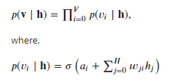
so, given current state of hidden units and weights, what is the probability of generating [1.0, 0.0, 0.0, 1.0, 0.0, 0.0, 0.0] in reconstruction phase, based on the above probability distribution function?

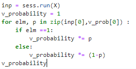
Now we have to calculate how similar X and V vectors are? The reconstructed values most likely will not look like the input vector because our network has not trained yet. Our objective is to train the model in such a way that the input vector and reconstructed vector to be same. Therefore, based on how different the input values look to the ones that we just reconstructed, the weights are adjusted.

Conclusion

Restricted Boltzmann Machine is generative models. An interesting aspect of an RBM is that the data does not need to be labelled. This turns out to be very important for real-world data sets like photos, videos, voices, and sensor data — all of which tend to be unlabeled. Rather than having people manually label the data and introduce errors, an RBM automatically sorts through the data, and by properly adjusting the weights and biases, an RBM is able to extract the important features and reconstruct
the input

I hope this article helped you to get the basic understanding Of Restricted Boltzmann Machine (RBM). I think it will at least provides a good explanation of steps involve in RBM.